Gradient Tree Boosting: XGBoost vs. LightGBM vs. CatBoost (Part 2)

Photo by Maxi am Brunnen on Unsplash

In Part 1, we have discussed about the basic algorithm of Gradient Tree Boosting.

Let’s start Part 2 today. We are going to focus on the competing algorithms in Gradient Tree Boosting: XGBoost, CatBoost and LightGBM. By reading the passage below, you will know the answers to the following questions for these 3 algorithms:

1. How does it handle missing values in splitting the nodes?

2. How does it handle categorical features in splitting the nodes?

3. How efficient it is to split nodes?

Xgboost

XGBoost was developed in 2014 by Tianqi Chen, who was then a PhD student in University of Washington (and will join Carnegie Mellon University as an Assistant Professor this Fall). This algorithm became famous in 2016 and now one of the de-facto tools for data scientists. To answer the three questions for XGBoost in short:

1. KEEP missing values as they are. When splitting a node, XGBoost compares the two scenarios where the missing values were put to right node and the left node; then selects the method which minimizes the loss function.

2. CANNOT handle categorical features. Need to convert categorical features to numeric, otherwise there will be errors.

3. RELATIVELY efficient, as XGBoost uses a less intensive way to find splitting points for nodes, and also parallel computation.

1. Sparse-aware Split Finding (How to Treat Missing Values)

Figure 1. Example of Sparse-aware Split Finding

The way that XGBoost handles missing values in split finding is pretty straightforward: just try! Put those missing values in the left and in the right of each split point, and then compare all the scenarios to find the one which reduces the loss function most.

Figure 1 shows an example where there is one missing value in the feature Age. When using Age in split finding, there are 2 split point candidates: 40 and 80. Combining the ways to treat the missing values, there will be 4 scenarios. Referring to Equation (7) in Part 1 of this series, we can use \Delta S to represent the improvement of node splitting. By comparing \Delta S under these 4 scenarios, we will know which is the optimal split point and also which node to put the missing value.

2. Split Finding Algorithm

When there are a limited number of split point candidates, XGBoost uses Extract Greedy Algorithm to find optimal split points. It enumerates over all the possible splits (values) of all the features.

However, when there are numerous split point candidates, the algorithm above is too costly in computation and requires large memory space. In this scenario, XGBoost uses Weighted Quantile Sketch in Approximate Algorithm to expedite the calculation. We will talk about the general, but not the details of Weighted Quantile Sketch here. Please watch this video or read Tianqi’s notes if you are interested in the details.

Figure 2 shows an example of Approximate Algorithm. With very few possible split points, take them all as split point candidates will be OK (Scenario 1). With too many possible split points (e.g. continuous variables), Approximate Algorithm can be used to find split point candidates. One common way is to use different percentiles of the feature.

Figure 2. Example of Approximate Algorithm

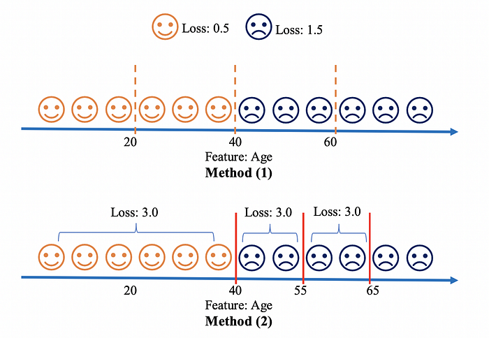
However, not all percentiles are equally important in split finding. Figure 3 points out a possible way to improve split finding in Approximate Algorithm, in the spirit of Weighted Quantile Sketch. Before using Age to split nodes, the sample is re-ordered by Age, the loss is computed for all the observations and is then aggregated to the level of different Ages. Method (1) shows the normal way of split finding: an equal proportion of observations distributed between different split points. But this splitting method does not reduce the total loss function efficiently. Apparently, setting a splitting point at Age 20, which is among the 6 points already with very small losses, cannot reduce much in the total loss function.

We’d better set more splitting points in the place where the loss is high, and less splitting points where the loss is low, shown in Method (2) of Figure 3. This is the spirit of Weighted Quantile Sketch. The split point is selected to make the similar sum of loss for the observations in different intervals.

Figure 3. Example of Weighted Quantile Sketch

CatBoost

CatBoost (Categorical Boosting) was first introduced by Yandex in 2017. To answer the three questions for CatBoost in short:

1. CANNOT handle missing values. Need to impute the missing values.

2. TREAT categorical variables well, with many methods available: e.g. One-Hot-Encode (much faster in CATBOOST), target statistics, frequency statistics as well as different combinations of features as splitting points.

3. VERY efficient, as CatBoost is more efficient in dealing with categorical variables besides the advantages of XGBoost.

1. Treatment of Categorical Features: Target Statistics

Two popular ways to deal with categorical features in algorithm are:

• One-hot encoding: Appropriate for low-cardinality categorical feature. Drawback: high-cardinality categorical features use very large memory space, and cause insufficient training examples.
• Target statistics: use target values to replace each level of categorical feature. Appropriate for categorical features of any cardinality. Drawback: target leakage (will be discussed below)

We focus on the method of Target Statistics (TS) in treating categorical features here. The basic idea of TS is to use the expected target value of each category to replace the categorical feature. That is, computationally, for any i­-th observation, its value of the categorical feature k will be replaced with the average target value of all the observations with the same categorical value as its:

This method has one problem: what if the denominator is zero? For example, when developing a model, the test set has a new categorical value, which is not in the training set. (The data processing of the test set should be independent of the training set, as if they don’t known the existence of each other).

1.1 Greedy TS

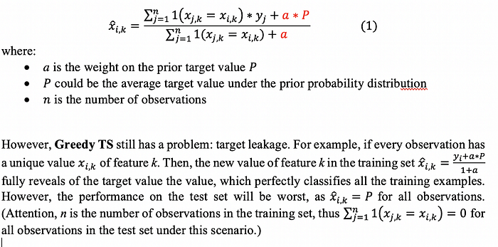
Greedy TS solves this problem by introducing a parameter a in the equation:

1.2 Ordered TS

To solve this problem, CatBoost uses Ordered TS (there are other methods such as Holdout TS, Leave-one-out TS, please read the original paper of CatBoost for more details). The basic idea of Ordered TS is:

But if we simply use Equation (2) to replace the categorical value, there is one problem: the proceeding observations have their TS with much larger variances than the subsequent ones. Ordered TS has made an improvement by using permutations, as shown in Figure 4.

Figure 4 shows an example of using Ordered TS to replace the categorical value of 3rd observation (the blue ball with the red circle). In the normal way to calculate the new value for 3rd observation, we only look at the two observations (set S) in front of it and apply Equation (2). Ordered TS uses the same logics but after reshuffle all the observations. Then, to calculate the new value for 3rd observation, we will look at the four observations (set S_/sigma) and apply Equation (2).

Figure 4. Example of Ordered TS

To put it mathematically, Ordered TS computes the new values for categorical variables in the following steps:

• Step 1: For each categorical variable k and each observation i, take a random permutation denoted as \sigma = (\sigma_1, \sigma_2, …, \sigma_n). It is the index order for the reshuffled observations. For example, in Figure 4 the original order of observations is (1, 2, 3, …, n), after the reshuffle it is (n, 1, 5,…, 4).
• Step 2: Apply Equation (2) to the new permutation of the observations. The modified equation will be:

2. Problem of Prediction Shift

The problem of Prediction Shift is first revealed in CatBoost. What does Prediction Shift mean? In Boosting, if fitting many models on the same training dataset which will be used in prediction, it will cause a biased estimation, i.e. Prediction Shift.

In the paper of CatBoost, it gives a concrete example to show Prediction Shift (Read the original paper for more details):

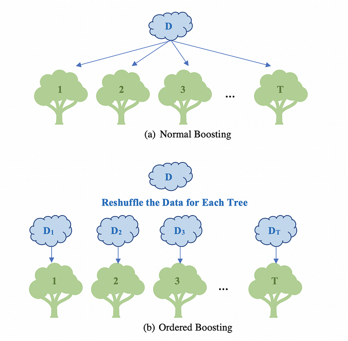
To solve the problem of Prediction Shift, CatBoost uses Ordered Boosting. Figure 5 shows the idea of Order Boosting. Figure 5 (a) is the normal way Boosting used to train models, which leads to Prediction Shift. Compared with that, Figure 5 (b) shows Ordered Boosting: each model is trained on a reshuffled dataset. Within each tree, there will be n different supporting models M_1, M_2, …, M_n where each supporting model Mi is trained only on first (i-1) observations. To compute the residual for observation i, we only use model M_{i-1}. (Read the original paper if you are interested in the details.)

Figure 5. Idea of Ordered Boosting

LightGBM

LightGBM was developed by Microsoft in 2017. It aims to make the algorithm efficient and scalable to deal with big data. LightGBM greatly reduces the data set by reducing the data size and feature numbers in splitting nodes (that is why it is called “light”). To answer the three questions for LightGBM in short:

1. KEEP missing values as they are. Treat them in the same way as XGBoost.

2. CAN treat categorical variables, but only in two ways one-hot-encoding or label-encoding.

3. MOST efficient, as LightGBM reduces the sample size and the number of features in training by Gradient-based One-Side Sampling (GOSS) and Exclusive Feature Bundling (EFB), and also saves time by using leaf-wise growth strategy (we won’t cover it in this topic). However, its efficiency is at the cost of accuracy.

1. Reduce Data Size (Gradient-based One-Side Sampling, GOSS)

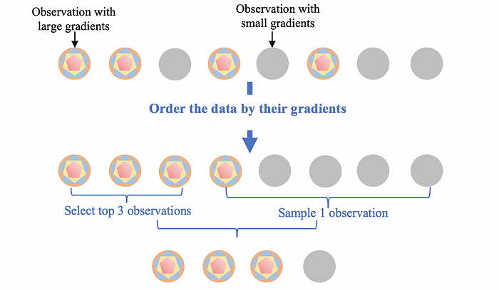
The fundamental reason why it is possible to reduce data size is that not all observations are equally important in training. The idea of Gradient-based One-Side Sampling (GOSS) is that the observations with the larger gradients (i.e. residuals) play an more important role in training. Thus, GOSS down samples the data by looking at their gradients. However, if simply discard the observations with small gradients, it will alter the data distribution and hurt the accuracy of the training model. To avoid that, besides select a number of observations with the large gradients, GOSS samples the observations with the small gradients, and then amplify their information gain with different factors.

Figure 6. Example of GOSS

Figure 6 shows an example of GOSS. In details, it is done in the following steps:

• Step 1: Compute the gradients (i.e. residuals) of all the observations.
• Step 2: Sort the observations according to their gradients.
• Step 3: Select top a *100% observations.
• Step 4: Randomly sample b * 100% observations from the rest of data.
• Step 5: when calculate the information gain, amplify the randomly selected data (i.e. in Step 4) by (1-a)/b.

2. Reduce Feature Numbers (Exclusive Feature Bundling, EFB)

The idea of Exclusive Feature Bundling (EFB) is straightforward. The big data are usually high-dimensional and very sparse thus many features could be almost mutually exclusive. We can bundle these exclusive features together as “one feature” in splitting nodes, by allowing some level of conflicts. It uses the algorithm related to graph to reduce the complexity. We won’t discuss it in this topic. Please read the original paper if interested in the details.

Reference

1. XGBoost Part 4: Crazy Cool Optimizations. https://www.youtube.com/watch?v=oRrKeUCEbq8
2. XGBoost: A Scalable Tree Boosting System Supplementary Material. https://homes.cs.washington.edu/~tqchen/data/pdf/xgboost-supp.pdf
3. Chen, T., & Guestrin, C. (2016, August). Xgboost: A scalable tree boosting system. In Proceedings of the 22nd acm sigkdd international conference on knowledge discovery and data mining (pp. 785–794).
4. Prokhorenkova, L., Gusev, G., Vorobev, A., Dorogush, A. V., & Gulin, A. (2018). CatBoost: unbiased boosting with categorical features. In Advances in neural information processing systems (pp. 6638–6648).
5. Ke, G., Meng, Q., Finley, T., Wang, T., Chen, W., Ma, W., … & Liu, T. Y. (2017). Lightgbm: A highly efficient gradient boosting decision tree. In Advances in neural information processing systems (pp. 3146–3154).